Pre-requisites
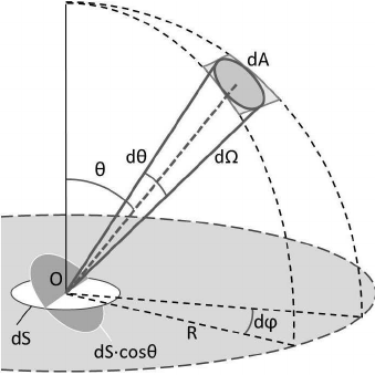
Solid Angle
In two dimensions, an angle of $2π$ radians covers the whole unit circle. Extending this to three dimensions, a solid angle of $4π$ steradians would cover the whole area of the unit sphere.
Radiometry
Radiometric quantities exist for measuring various aspects of electromagnetic radiation: overall energy, power (energy over time), and power density with respect to area, direction, or both.
energy Q: sources of illumination emit photons, each of which is at a particular wavelength and carries a particular amount of energy. A photon at wavelength $\lambda$ carries energy.
where $c$ is the speed of light, and $h$ is Planck’s constant.
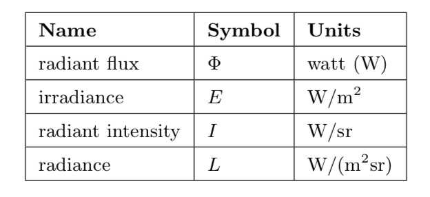
radiant flux $\Phi$: the basic unit in radiometry. Radiant flux is the flow of radiant energy over time—power—measured in watts (W).
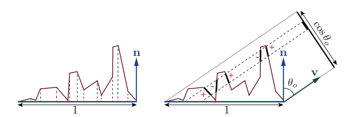
irradiance E: the density of radiant flux with respect to area. It is measured in watts per square meter. This area is measured in a plane perpendicular to the ray. If radiance is applied to a surface at some other orientation, then a cosine correction factor must be used.
radiant intensity I: flux density with respect to direction—more precisely, solid angle.
radiance L: measure of electromagnetic radiation in a single ray. More precisely, it is defined as the density of radiant flux with respect to both area and solid angle.
These quantities are summarized below.
The purpose of evaluating a shading equation is to compute the radiance along a given ray, from the shaded surface point to the camera.
Photometry
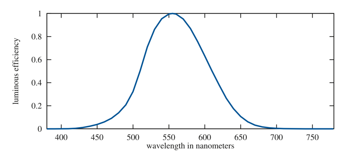
Radiometry deals purely with physical quantities, without taking account of human perception. A related field, photometry, is like radiometry, except that it weights everything by the sensitivity of the human eye. The results of radiometric computations are converted to photometric units by multiplying by the CIE photometric curve, a bell-shaped curve centered around 555 nm that represents the eye’s response to various wavelengths of light . Below is the photometric curve.
Subsurface Scattering
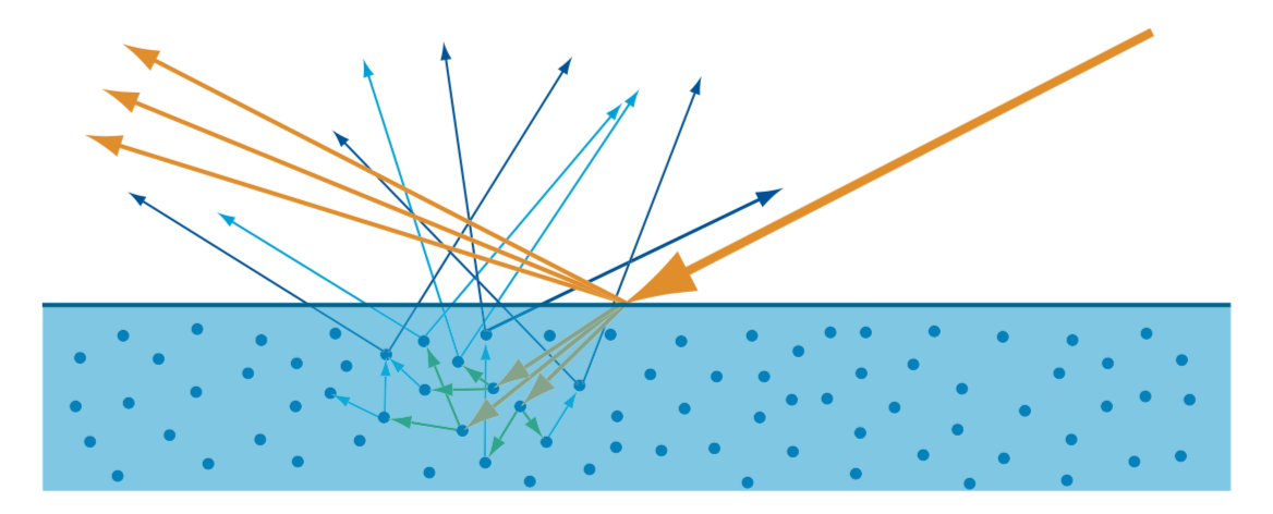
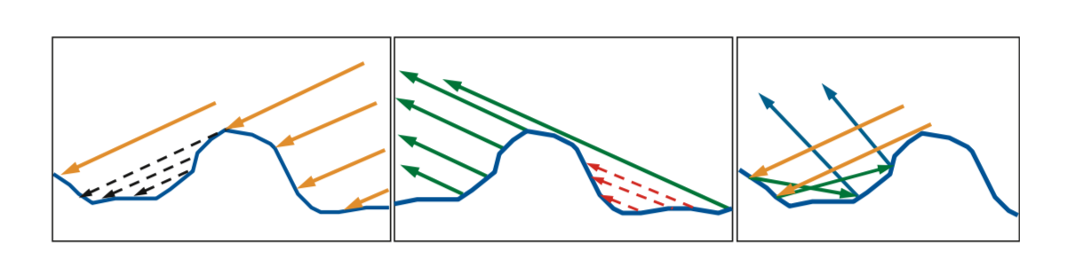
This subsurface-scattered light exits the surface at varying distances from the entry point. The distribution of entry-exit distances depends on the density and properties of the scattering particles in the material. The relationship between these distances and the shading scale (the size of a pixel, or the distance between shading samples) is important. If the entry-exit distances are small compared to the shading scale, they can be assumed to be effectively zero for shading purposes. This allows subsurface scattering to be combined with surface reflection into a local shading model, with outgoing light at a point depending only on incoming light at the same point. Since subsurface-scattered light has a significantly different appearance than surface reflected light, it is convenient to divide them into separate shading terms. The specular term models surface reflection, and the diffuse term models local subsurface scattering. If the entry-exit distances are large compared to the shading scale, then specialized rendering techniques, called global subsurface scattering techniques, are needed to capture the visual effect of light entering the surface at one point and leaving it from another.
Bidrectional reflectance distribution function
Physically based rendering comes down to computing the radiance entering the camera along some set of view rays. For a given view ray the quantity we need to compute is $L_{i}(c,−v)$, where $c$ is the camera position and $−v$ is the direction along the view ray. If we assume that there are no participating media present, where participating media means medium that a ray travel through, does affect radiance via absorption or scattering, then the radiance entering the camera is equal to the radiance leaving the closest object surface in the direction of the camera:
where $p$ is the intersection of the view ray with the closest object surface. Now focus on local reflectance phenomena, which redirect light hitting the currently shaded point back outward. These phenomenas include surface reflection as well as local subsurface scattering and depend only the incoming light direction $l$ and the outgoing view direction $v$. Local reflectance is quantified by the birectional reflectance distribution function(BRDF), denoted as $f(l,v)$, which was defined by Fred Nicodemus around 1965:
We can now get the reflectance equation:
The laws of physics impose two constraints on any BRDF.
- The first constraint is Helmholtz reciprocity, which means that the input and output angles can be switched and the function value will be the same:
- The second constraint is conservation of energy—the outgoing energy cannot be greater than the incoming energy.
The directional-hemispherical reflectance $R(l)$ is a function related to the BRDF. It can be used to measure to what degree a BRDF is energy conserving.
And a similar but in some sense opposite function, hemispherical-directional reflectance R(v) can be similarly defined:
If the BRDF is reciprocal, then the hemispherical-directional reflectance and the directional-hemispherical reflectance are equal. The value of the directional-hemispherical reflectance $R(l)$ must always be in the range [0, 1], as a result of energy conservation. A reflectance value of 0 represents a case where all the incoming light is absorbed or otherwise lost. If all the light is reflected, the reflectance will be 1.
Fresnel Reflectance
The Fresnel equations describe the dependence of $F$ on $θ_{i}$, $n_{1}$, and $n_{2}$. The value $n_{1}$ is the refractive index of the substance “above” the interface, where incident and reflected light propagate, and $n_{2}$ is the refractive index of the substance “below” the interface, where the refracted light propagates. the Fresnel reflectance is always notated as $F(n,l)$. When light perpendicular to the surface $(l = n)$, $F(n,l)$ has a value that is a property of the substance. This value, $F_{0}$, can be thought of as the characteristic specular color of the substance. The case when $(l=n)$ is called normal incidence. As the light strikes the surface at increasingly glancing angles, the value of $F(n,l)$ will tend to increase, reaching a value of 1 for all frequencies (white) at angle 90. The increase in reflectance at glancing angles is often called the Fresnel effect.
Schlick gives an approximation of Fresnel reflectance.
The refractive index can also be used to compute $F_{0}$ with the following equation:
- Dielectrics have fairly low values for $F_{0}$—usually 0.06 or lower. This low reflectance at normal incidence makes the Fresnel effect especially visible for dielectrics. The optical properties of dielectrics rarely vary much over the visible spectrum, resulting in colorless reflectance values.
- Metals have high values of $F_{0}$—almost always 0.5 or above. Some metals have optical properties that vary over the visible spectrum, resulting in colored reflectance values.
Microfacet Theory
An important property of a microfacet model is the statistical distribution of the microfacet normals $m$. This distribution is defined by the surface’s normal distribution function, or NDF. We will use $D(m)$ to refer to the NDF in equations.
Integrating $D(m)$ over the entire sphere of microfacet normals gives the area of the microsurface.
The integral is over the entire sphere, represented here by $\Theta$. More generally, the projections of the microsurface and macrosurface onto the plane perpendicular to any view direction $v$ are equal:
Most surfaces have NDFs that show a strong peak at the macroscopic surface normal $n$. More generally, we always use an alternative way of relating the projected microfacet areas to the projected macrogeometry area: The sum of the projected areas of the visible microfacets is equal to the projected area of the macrosurface. To do that, we can define a masking function $G1(m, v)$, which gives the fraction of microfacets with normal $m$ that are visible along the view vector $v$.
Dot product in the above equation is clamped to zero by the $x^{+}$ notation.
Given a microgeometry description including a micro-BRDF $f_{\mu }(l, v, m)$, normal distribution function $D(m)$, and masking function $G_{1}(m, v)$, the overall macrosurface BRDF can be derived:
This integral is over the hemisphere $\Omega$ centered on $n$. Instead of the masking function $G_{1}(m, v)$, the equation uses the joint masking-shadowing function $G_{2}(l, v, m)$. It gives the fraction of microfacets with normal $m$ that are visible from two directions: the view vector $v$ and the light vector $l$.
BRDF Models for Surface Reflection
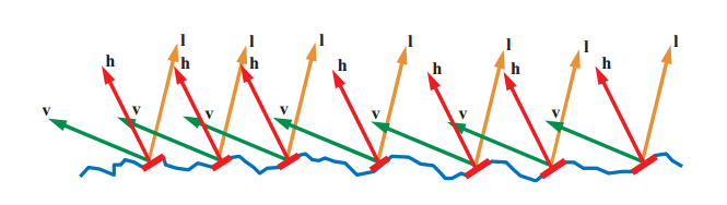
In the case of specular surface reflection, each microfacet is a perfectly smooth Fresnel mirror. This means that the micro-BRDF $f_{\mu }(l, v, m)$ for each facet is equal to zero unless $v$ is parallel to the reflection of $l$. It indicates that surface normal aligned with the half vector $h$, participate in the reflection of light from the incoming light vector $l$ to the view vector $v$.
Since it collapses the integral into an evaluation of the integrated function at $m = h$. Doing so yields the specular BRDF term: Details on the derivation can be found in publications by Walter et al.
Normal Distribution Functions
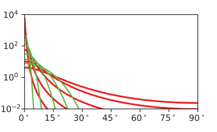
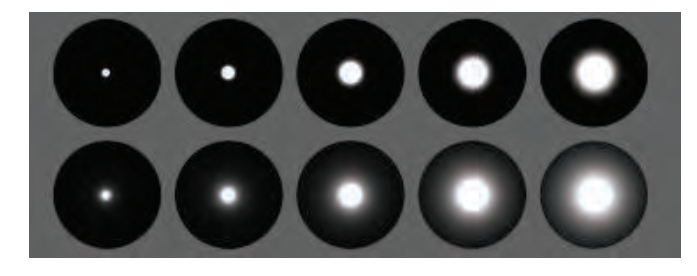
The GGX distribution is isotropic normal distribution function, started spreading across the film and game industries, and today it likely is the most often-used distribution in both. The GGX distribution is: Comparison of GGX(red) and Beckmann(green) distributions for different $\alpha $ value.
These same values have been used in the spheres rendered on the below image. The top row uses the Beckmann NDF and the bottom row uses GGX.
Reference
- Real-Time Rendering Fourth Edition
- Physically Based Rendering: From Theory to Implementation