Light Scattering Theory

Properties of Volumes

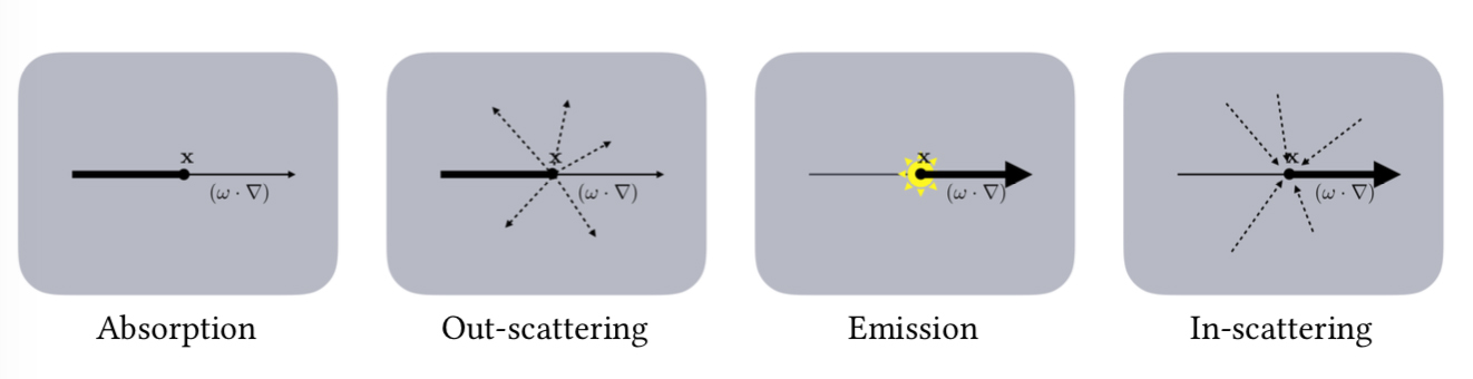
There are four types of events that can affect the amount of radiance propagating along a ray through a medium.

• Absorption expressed with the coefficient $\sigma _{a}(x)$, describes the collision when a photon is absorbed by the volume. Physically, the photon energy is transferred into some volume particle internal energy such as translational or vibrational modes in molecules or more generally into heat.
• Scattering A scattering collision $\sigma _{s}(x)$ scatters the photon into a different direction defined by the phase function. The radiance value carried by the photon does not change with a scattering collision; any change in radiance is modeled with absorption and emission.
• Phase Function The phase function $f_{p}(x,\omega ,\omega’)$ is the angular distribution of radiance scatterd and is usually modeled as a 1D function of the angle $\theta$ between the two directions $\omega$ and $\omega’$. Phase functions need to be normalized over the sphere:

An important property of phase functions — similar to BSDFs — is reciprocity. We need to be able to interchange the directions without changing the value of the phase function. Isotropic volumes have an equal probability of scattering incoming light in any direction, and have an associated phase function:

Anisotropic volumes can exhibit complicated phase functions. As an alternative, in production volume rendering, the most widely used phase function is the Henyey-Greenstein phase function:

where $-1<g<1$. The single parameter $g$ can be understood as the average cosine of the scattering directions, and controls the asymmetry of the phase function. It can model backwards scattering($g<0$), isotropic scattering($g=0$), and forward scattering($g>0$).

• Emission Volumes emit radiance in a volumetric fashion, but otherwise behave exactly like another light source. The emitted radiance is expressed as radiance field $L_{e}(x, \omega)$. In any real-world scenario, volumes do not emit directionally, and $L_{e}(x, \omega )$ is the same in all directions $\omega $.

Extinction defines the loss of radiance due to both absorption and scattering, and we can model that loss with a single coefficient $\sigma _{t} = \sigma _{a}+\sigma {s}$. The single scattering albedo $\alpha = \frac {\sigma _{s}}{\sigma _{t}}$ is defined in addition to the extinction to unambiguously define volume properties. $\alpha $ has a similar meaning to the surface albedo: both are a measure of overall reflectivity that determines the amount of scattered radiance. An $\alpha = 0$ means that all radiance is absorbed and an $\alpha = 1$ means that no absorption occurs and we have lossless scattering.

Radiative Transfer Equation

The distribution of radiance in volumes is defined by the radiative transfer equation, which defined by Chandrasekhar. It describes the equilibrium radiance field $L(x, \omega )$ parametrized by position $x$ and the direction $\omega $.

• Absorption For an exemplary radiance beam $L(x, \omega )$, starting at $x$ with direction $\omega $, the derivative of the radiance in the direction of $\sigma $ is proportional to the radiance at that point:

• Out-Scattering The exemplary radiance beam $L(x, \omega )$ also loses radiance due to out-scattering into other directions than its own direction. The loss is again proportional to the radiance $L(x, \omega )$ with the proportionality factor being the scattering coefficient $\sigma _{s}$:

• Emission. Emission is a seperate radiance field $L_{e}(x, \omega )$ that defines the radiance added to the radiance field $L(x, \omega )$:

• In-Scattering. In-Scattering is a contribution from the out-scattering of all of the other directions $\omega’$ at x:

where $S^{2}$ denotes the spherical domain around the position $x$. The $\sigma _{s}$ in front of the integral models the scattering of the incoming radiance from all of the directions similar to the $\sigma _{s}$ in the out-scattering equation.

• Assembling. Now add up all constituent terms. Due to their fundamental similarity, absorption and out-scattering can be combined into the extinction coefficient $\sigma _{t}(x)$:

where $L_{s}(x, \omega) = \int _{S^{2}}f_{p}(x, \omega , \omega')L(x, \omega')d\omega'$ for simplification.

The Real-time Volumetric Cloudscapes of Horizon

Andrew Schneider and Nathan Vos introduce a voxel clouds system in the game Horizon Zero Dawn at SIGGRAPH 2015, as part of the Adavances in Real-time rendering Course.

Modeling

The modeling approach uses ray marching to produce clouds. Rays march from the camera and sample noises and a set of gradients to define the cloud shapes. Layering Perlin noises of different frequencies in the sample procedure would make a very procedural looking clouds. So they introduce Worley noice as an offset to dilate Perlin noise. This would keep connectedness of Perlin noise but add some billowy shapes to it, which is referred as ‘Perlin-Worley’ noise.

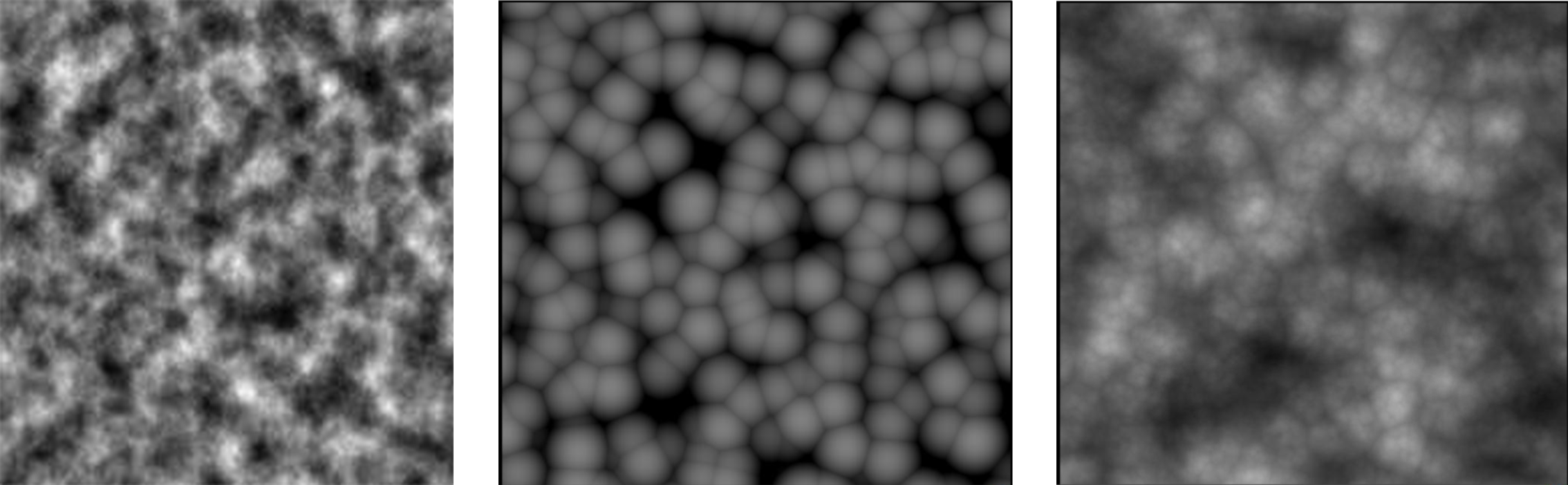
Two 3d textures and one 2d texture are used in the system. The first 3D texture with 128^2 resolution define the base shape for the clouds. And its first channel is the Perlin-Worley noise. The other three are Worley noise at increasing frequencies. The second 3D texture has three channels with 32^3 resolution, and uses Worley noise at increasing frequencies. This texture is used to add detail to the base cloud shape defined by the first 3D noise. The 2D texture has three channels with 128^2 resolution, and uses curl noise, which is non-divergent and is used to fake fluid motion, distort cloud shapes and add a sense of turbulence. Three height gradients are preset for the major low altitude cloud types: stratus, cumulus and cumulonimbus, which are used to change the noise signal over altitude. And a value between 0 and 1 is also defined to tell how much cloud coverage at the sample position. The whole modeling approach follow the standard ray-march/sampler framework:

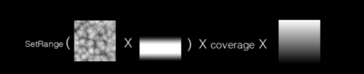
• Build a low frequency cloud base shape. Sample the first 3D texture and multiplying it by height signal; then multiply the result by the coverage and reduce density at the bottoms of the clouds.

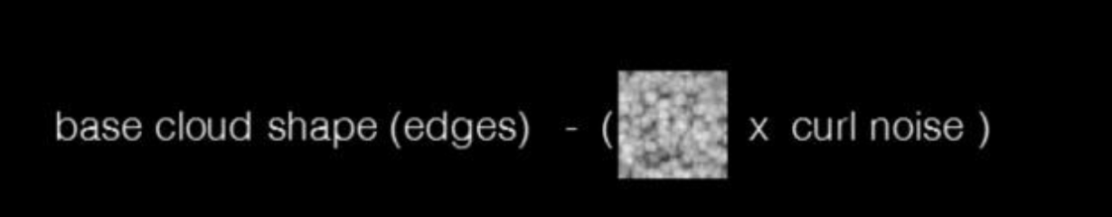
• Add high frequency detail and distortion. Erode the base cloud shape by subtracting the second 3D texture at the edge of the cloud. Also distort the second noise by the 2D curl noise to fake the swirly distortions from atmospheric turbulence.

• Use a set of presets for each cloud type to control density over height and cloud coverage. These are driven by the weather simulation.

  Lighting

  The lighting of clouds can be described as the following equation:

where $d$ denotes the cloud depth, and $r$ means the absorption increasing for rain clouds.

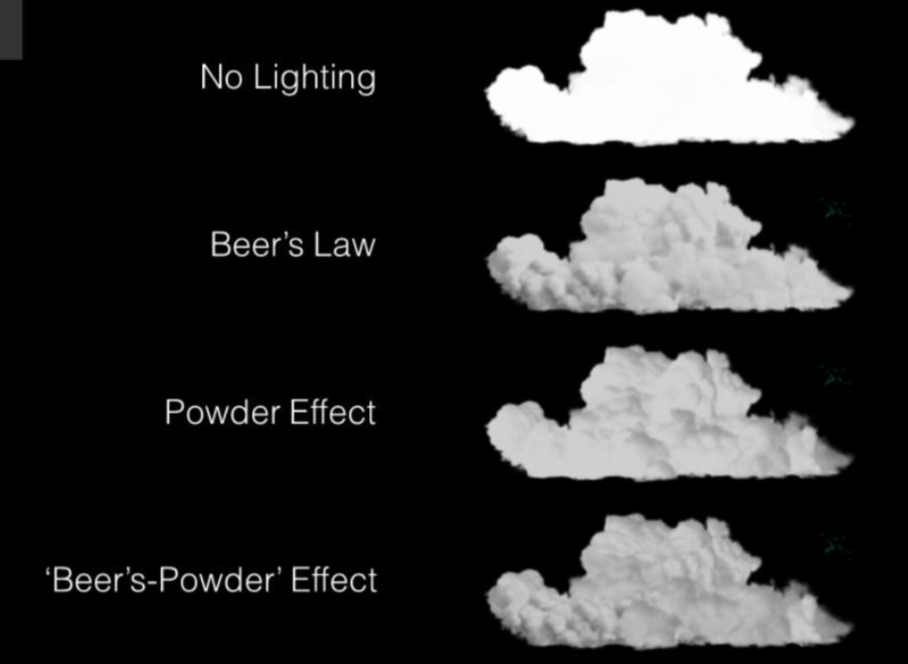
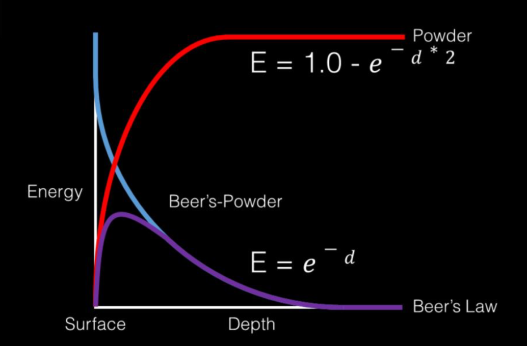
• Beer’s Law. The first component $e_{-dr}$ is Beer’s Law, which states that the amount of light reaching a point can be determined by the optical thickness of the medium that it travels through.
• Henyen-Greenstein. The second component $f_{hg}$ helps reproduce anisotropy in cloud lighting, which is introduced in the previous light scattering theory section.
• Powder Effect. There is a property in clouds that points inside would receive more in scattered light than ones near surface, which is a similar effect in piles of powdered sugar. So a powder curve can be used to approximate such effect.

Reference

1. Julian F., Magnus W., Christopher K., Ralf H., Production Volume Rendering.
2. Andrew S., Nathan V., The Real-time Volumetric Cloudscapes of Horizon.